InClass Ex4

In Class Exercise 4

pacman::p_load(tidyverse, ggstatsplot, rstantools)

Tidyverse

ggplot2, dplyr, tidyr, readr, purrr, tibble, stringr, forcats are in the package of Tidyverse.

exam <- read_csv("data/Exam_data.csv")

set.seed(1234)

Parametric Testing

p <- gghistostats(
  data = exam,
  x = ENGLISH,
  conf.level = 0.95,
  type = "parametric",
  test.value=60,
  bin.args = list(color="black",
                  fill = "grey50",
                  alpha=0.7),
  normal.curve = FALSE,
  normal.curve.args = list(linewidth = 2),
  xlab = "English scores"
)

Populating the statistics results from above

extract_stats(p)

$subtitle_data
# A tibble: 1 × 15
     mu statistic df.error  p.value method            alternative effectsize
  <dbl>     <dbl>    <dbl>    <dbl> <chr>             <chr>       <chr>     
1    60      8.77      321 1.04e-16 One Sample t-test two.sided   Hedges' g 
  estimate conf.level conf.low conf.high conf.method conf.distribution n.obs
     <dbl>      <dbl>    <dbl>     <dbl> <chr>       <chr>             <int>
1    0.488       0.95    0.372     0.603 ncp         t                   322
  expression
  <list>    
1 <language>

$caption_data
# A tibble: 1 × 16
  term       effectsize      estimate conf.level conf.low conf.high    pd
  <chr>      <chr>              <dbl>      <dbl>    <dbl>     <dbl> <dbl>
1 Difference Bayesian t-test     7.16       0.95     5.54      8.75     1
  prior.distribution prior.location prior.scale    bf10 method         
  <chr>                       <dbl>       <dbl>   <dbl> <chr>          
1 cauchy                          0       0.707 4.54e13 Bayesian t-test
  conf.method log_e_bf10 n.obs expression
  <chr>            <dbl> <int> <list>    
1 ETI               31.4   322 <language>

$pairwise_comparisons_data
NULL

$descriptive_data
NULL

$one_sample_data
NULL

$tidy_data
NULL

$glance_data
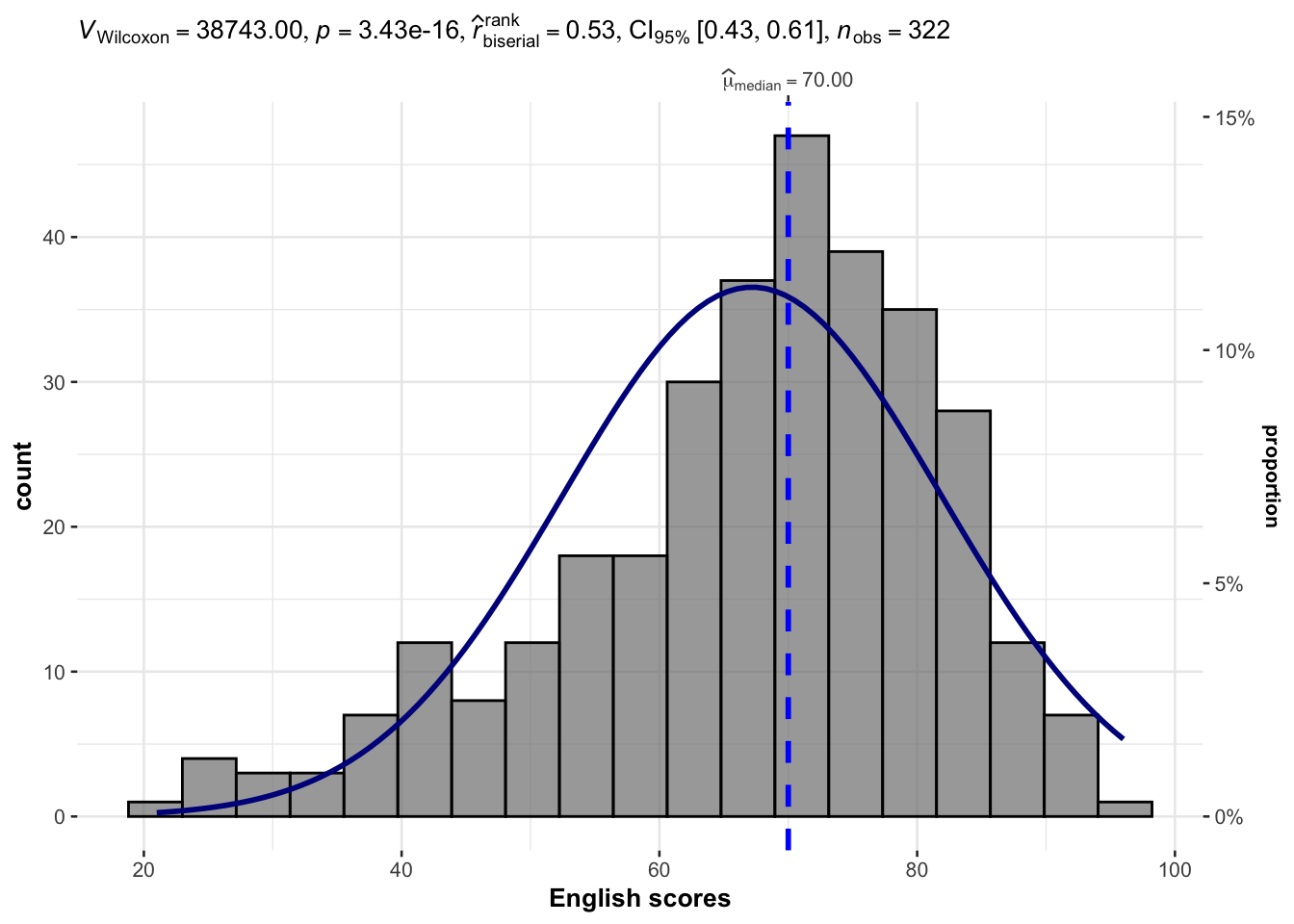
NULL

Non Parametric - Wilcoxon

gghistostats(
  data = exam,
  x = ENGLISH,
  conf.level = 0.95,
  type = "np",
  test.value=60,
  bin.args = list(color="black",
                  fill = "grey50",
                  alpha=0.7),
  normal.curve = TRUE,
  normal.curve.args = list(linewidth = 1, color="darkblue"),
  xlab = "English scores"
)

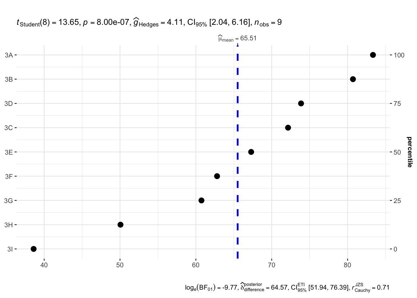
ggdotplotstats(
  data = exam,
  x = ENGLISH,
  y = CLASS,
  title = "",
  xlab = ""
)

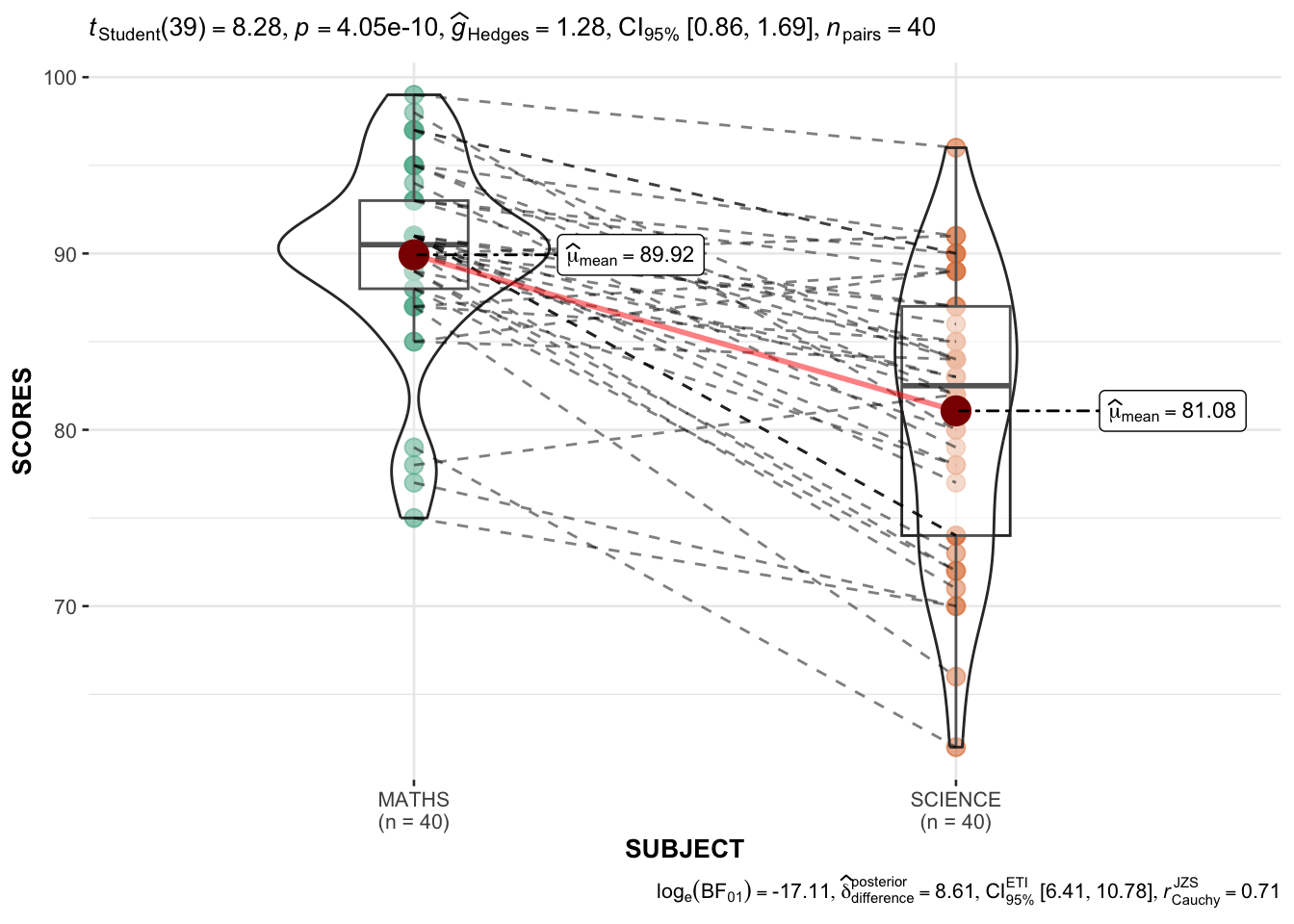
Pivot Table first

exam_long <-  exam %>%
  pivot_longer(
    cols = ENGLISH:SCIENCE,
    names_to = "SUBJECT",
    values_to = "SCORES") %>%
  filter(CLASS == "3A")

ggwithinstats(
  data = filter(exam_long,
                SUBJECT %in%
                    c("MATHS", "SCIENCE")),
  x = SUBJECT,
  y = SCORES,
  type = "p"
)

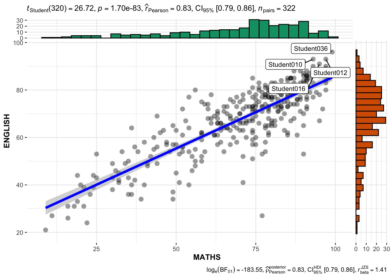
Scatterplot & Histogram

ggscatterstats(
  data = exam,
  x = MATHS,
  y = ENGLISH,
  marginal = TRUE,
  label.var = ID,
  label.expression = ENGLISH > 90 & MATHS > 90,
  )

10.4 Visualising Models

pacman::p_load(easystats)

easystats package

pacman::p_load(readxl, performance, parameters, see)

Links:

https://indrajeetpatil.github.io/ggstatsplot/ Robust excludes outliers in analysis